Analyzing the Parker Solar Probe flybys

1. Modulus of the exit velocity, some features of Orbit #2

First, using the data available in the reports, we try to compute some of the properties of orbit #2. This is not enough to completely define the trajectory, but will give us information later on in the process.

from astropy import units as u

T_ref = 150 * u.day
T_ref

$150 \; \mathrm{d}$

from poliastro.bodies import Earth, Sun, Venus

k = Sun.k
k

$1.3271244 \times 10^{20} \; \mathrm{\frac{m^{3}}{s^{2}}}$

import numpy as np

\[T = 2 \pi \sqrt{\frac{a^3}{\mu}} \Rightarrow a = \sqrt[3]{\frac{\mu T^2}{4 \pi^2}}\]

a_ref = np.cbrt(k * T_ref ** 2 / (4 * np.pi ** 2)).to(u.km)
a_ref.to(u.au)

$0.55249526 \; \mathrm{AU}$

\[\varepsilon = -\frac{\mu}{r} + \frac{v^2}{2} = -\frac{\mu}{2a} \Rightarrow v = +\sqrt{\frac{2\mu}{r} - \frac{\mu}{a}}\]

energy_ref = (-k / (2 * a_ref)).to(u.J / u.kg)
energy_ref

$-8.0283755 \times 10^{8} \; \mathrm{\frac{J}{kg}}$

from poliastro.twobody import Orbit
from poliastro.util import norm

from astropy.time import Time

flyby_1_time = Time("2018-09-28", scale="tdb")
flyby_1_time

<Time object: scale='tdb' format='iso' value=2018-09-28 00:00:00.000>

r_mag_ref = norm(Orbit.from_body_ephem(Venus, epoch=flyby_1_time).r)
r_mag_ref.to(u.au)

$0.72573132 \; \mathrm{AU}$

v_mag_ref = np.sqrt(2 * k / r_mag_ref - k / a_ref)
v_mag_ref.to(u.km / u.s)

$28.967364 \; \mathrm{\frac{km}{s}}$

2. Lambert arc between #0 and #1

To compute the arrival velocity to Venus at flyby #1, we have the necessary data to solve the boundary value problem.

d_launch = Time("2018-08-11", scale="tdb")
d_launch

<Time object: scale='tdb' format='iso' value=2018-08-11 00:00:00.000>

ss0 = Orbit.from_body_ephem(Earth, d_launch)
ss1 = Orbit.from_body_ephem(Venus, epoch=flyby_1_time)

tof = flyby_1_time - d_launch

from poliastro import iod

((v0, v1_pre),) = iod.lambert(Sun.k, ss0.r, ss1.r, tof.to(u.s))

v0

$[9.5993373,~11.298552,~2.9244933] \; \mathrm{\frac{km}{s}}$

v1_pre

$[-16.980821,~23.307528,~9.1312908] \; \mathrm{\frac{km}{s}}$

norm(v1_pre)

$30.248465 \; \mathrm{\frac{km}{s}}$

3. Flyby #1 around Venus

We compute a flyby using poliastro with the default value of the entry angle, just to discover that the results do not match what we expected.

from poliastro.threebody.flybys import compute_flyby

V = Orbit.from_body_ephem(Venus, epoch=flyby_1_time).v
V

$[648499.74,~2695078.4,~1171563.7] \; \mathrm{\frac{km}{d}}$

h = 2548 * u.km

d_flyby_1 = Venus.R + h
d_flyby_1.to(u.km)

$8599.8 \; \mathrm{km}$

V_2_v_, delta_ = compute_flyby(v1_pre, V, Venus.k, d_flyby_1)

norm(V_2_v_)

$27.755339 \; \mathrm{\frac{km}{s}}$

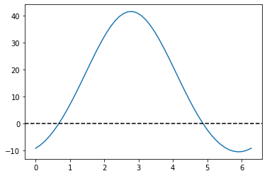
4. Optimization

Now we will try to find the value of \(\theta\) that satisfies our requirements.

def func(theta):
    V_2_v, _ = compute_flyby(v1_pre, V, Venus.k, d_flyby_1, theta * u.rad)
    ss_1 = Orbit.from_vectors(Sun, ss1.r, V_2_v, epoch=flyby_1_time)
    return (ss_1.period - T_ref).to(u.day).value

There are two solutions:

import matplotlib.pyplot as plt

theta_range = np.linspace(0, 2 * np.pi)
plt.plot(theta_range, [func(theta) for theta in theta_range])
plt.axhline(0, color="k", linestyle="dashed");

func(0)

-9.142672330001131

func(1)

7.09811543934556

from scipy.optimize import brentq

theta_opt_a = brentq(func, 0, 1) * u.rad
theta_opt_a.to(u.deg)

$38.598709 \; \mathrm{{}^{\circ}}$

theta_opt_b = brentq(func, 4, 5) * u.rad
theta_opt_b.to(u.deg)

$279.3477 \; \mathrm{{}^{\circ}}$

V_2_v_a, delta_a = compute_flyby(v1_pre, V, Venus.k, d_flyby_1, theta_opt_a)
V_2_v_b, delta_b = compute_flyby(v1_pre, V, Venus.k, d_flyby_1, theta_opt_b)

norm(V_2_v_a)

$28.967364 \; \mathrm{\frac{km}{s}}$

norm(V_2_v_b)

$28.967364 \; \mathrm{\frac{km}{s}}$

5. Exit orbit

And finally, we compute orbit #2 and check that the period is the expected one.

ss01 = Orbit.from_vectors(Sun, ss1.r, v1_pre, epoch=flyby_1_time)
ss01

0 x 1 AU x 18.8 deg (HCRS) orbit around Sun (☉) at epoch 2018-09-28 00:00:00.000 (TDB)

The two solutions have different inclinations, so we still have to find out which is the good one. We can do this by computing the inclination over the ecliptic - however, as the original data was in the International Celestial Reference Frame (ICRF), whose fundamental plane is parallel to the Earth equator of a reference epoch, we have change the plane to the Earth ecliptic, which is what the original reports use.

ss_1_a = Orbit.from_vectors(Sun, ss1.r, V_2_v_a, epoch=flyby_1_time)
ss_1_a

0 x 1 AU x 25.0 deg (HCRS) orbit around Sun (☉) at epoch 2018-09-28 00:00:00.000 (TDB)

ss_1_b = Orbit.from_vectors(Sun, ss1.r, V_2_v_b, epoch=flyby_1_time)
ss_1_b

0 x 1 AU x 13.1 deg (HCRS) orbit around Sun (☉) at epoch 2018-09-28 00:00:00.000 (TDB)

Let’s define a function to do that quickly for us, using the `get_frame <https://docs.poliastro.space/en/latest/api/safe/frames.html#poliastro.frames.get_frame>`__ function from poliastro.frames:

from astropy.coordinates import CartesianRepresentation, CartesianDifferential
from poliastro.frames import Planes
from poliastro.frames.util import get_frame


def change_plane(ss_orig, plane):
    """Changes the plane of the Orbit.

    """
    ss_orig_rv = ss_orig.get_frame().realize_frame(
        ss_orig.represent_as(CartesianRepresentation, CartesianDifferential)
    )

    dest_frame = get_frame(ss_orig.attractor, plane, obstime=ss_orig.epoch)

    ss_dest_rv = ss_orig_rv.transform_to(dest_frame)
    ss_dest_rv.representation_type = CartesianRepresentation

    ss_dest = Orbit.from_coords(ss_orig.attractor, ss_dest_rv, plane=plane)
    return ss_dest

change_plane(ss_1_a, Planes.EARTH_ECLIPTIC)

0 x 1 AU x 3.5 deg (HeliocentricEclipticIAU76) orbit around Sun (☉) at epoch 2018-09-28 00:00:00.000 (TDB)

change_plane(ss_1_b, Planes.EARTH_ECLIPTIC)

0 x 1 AU x 13.1 deg (HeliocentricEclipticIAU76) orbit around Sun (☉) at epoch 2018-09-28 00:00:00.000 (TDB)

Therefore, the correct option is the first one.

ss_1_a.period.to(u.day)

$150 \; \mathrm{d}$

ss_1_a.a

$82652115 \; \mathrm{km}$

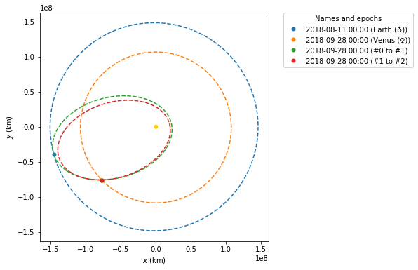
And, finally, we plot the solution:

from poliastro.plotting import StaticOrbitPlotter

frame = StaticOrbitPlotter()

frame.plot(ss0, label=Earth)
frame.plot(ss1, label=Venus)
frame.plot(ss01, label="#0 to #1")
frame.plot(ss_1_a, label="#1 to #2");